Friday, August 31, 2018

An Interview Question I Would be Horrible At

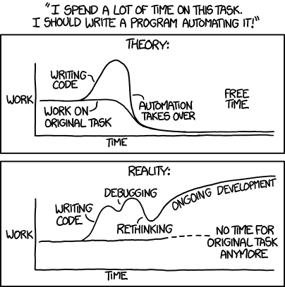
XKCD: Strengths and Weaknesses

Have you ever had programming/algorithm interview questions that require you to write code off the top-of-your-head without a keyboard at your fingertips, while in a stressful situation, away from your normal development environment?

I've had a few interviews like that in the past. I usually come up with all sorts of creative answers

... starting right after I finish the interview, as I'm driving away in my car, then hitting a peak the morning after (that's when I really shine!). During the actual interview, my apparent IQ drops by 1/3.

Maybe the reason I suck at "whiteboard coding" in interviews is that I don't practice it. It is nothing like what I actually do for a job, so I would need to suck it up and spend some time practicing "coding quizzes" to do well in such an interview. I would rather skip that and do real work instead.

Also, I have to admit another probable reason as well. I'm just not well-suited for it. I would characterize my general methodology as somewhat measured, thoughtful and methodical to offset my zany, intuitive, artsy tendencies. This is an unlikely teeter-totter balance honed from dauntless decades of determined dedication. Also, there is a certain amount of high-quality coffee required. This juggling act just does not mix well with interviews. Strengths are weaknesses.

Having said all that, I'm going to visit a worst-nightmare example of an interview question for "educational purposes":


THE INTERVIEW QUESTION

Given a list of n+2 numbers, with all numbers in the range of 1..n and all numbers unique except for two numbers which each occur twice, find the duplicate numbers. Use two different methods, each using no more than one loop. Compare and contrast the advantages and disadvantages of each.

To get warmed up, first let's start with the the easiest algorithm I can think of -- one that would be a FAIL because it uses two loops:

Method #1 Nested Loops


Use two loops to compare every list element to every other element. If two different elements are equal, then you have found the duplicate.

Python:
mylist = [1,2,3,3,4,5,6,6,7]
mylist_size = len(mylist)
for x in range (0, mylist_size):
    for y in range (x + 1, mylist_size):
        if mylist[x] == mylist[y]:
            print(mylist[x])

This method does not take advantage of all the provided information: that there are only two repeating elements and the elements are in the range 1..n. It is a more generic and flexible approach, which can adapt to an arbitrary number of repeating elements (not just two) and can also handle lists of numbers outside of the 1..n range. Such flexibility is valuable if the needs are likely to evolve over time, which is a valuable consideration in building real-world systems.

The performance is O(n²), so is directly proportional to the square of the list size (it will gobble up cpu/time). For example, a 1,000 item list only took 6 seconds on my laptop, but a 10,000 item list took over two minutes. I can estimate that a 100,000 item list would take 100 times longer (about 3 1/2 hours).

On a positive note, it requires minimal O(1) state (it will not gobble up disk/memory) and is the simplest of the three methods.

This does not scale out well as it is essentially a cartesian product. It would be problematic to distribute this across many compute nodes as you would need to copy/shuffle the list around quite a bit.

This approach is perhaps well-suited for implementations with tiny data (dozens to hundreds of rows tops), where the code-simplicity outweighs all other concerns. Maybe it is also useful as an example of What Not To Do.


Method #2 loop and dictionary


For the second attempt, let's try to actually provide a solution that will meet the requirements.

Use one loop and a dictionary to keep track of all elements in the list. When you see an element a 2nd time, then it is a duplicate.

Python:
mylist = [1,2,3,3,4,5,6,6,7]
mylist_size = len(mylist)

# create dictionary of counts
count_dict = {}
for x in range(0, mylist_size):
    # we have already seen this element, it is a duplicate
    if (mylist[x] in count_dict):
        print(mylist[x])
    else:
        # have not seen this element yet, so add to dictionary
        count_dict[mylist[x]] = 1


Like method #1, this method does not take advantage of all the provided information: that there are only two repeating elements and that the numbers are in the range 1..n. Similar to method #1 it is also a more generic and flexible approach that can handle similar adaptations.

This approach performs O(n) for cpu/time but also requires O(n) state (memory/disk -- whichever) for the dictionary, so is more efficient in terms of cpu/time and state than method #1, but is more complicated. There are variations that reduce state a little by keeping a dictionary of hashes, or modifying the list itself to mark duplicates.

A 100,000 item list took about 6 seconds on my laptop (I WAG this is ~2,000 times faster than method 1 for the same sized list). I did not bother to measure the memory used by the dictionary, but that would be the limit one would hit first using this method.

This approach is straightforward to scale out across many nodes as you can easily partition out the work and the reassemble the results.

I would generally default to this approach as the best-balanced of the three methods here.


Method #3 system of equations


Create a system of equations to solve for the two repeating values.

given:
    S is sum of all numbers in the list
    P is the product of all numbers in the list
    X and Y are the duplicate numbers in the list
    the sum of integers from 1 to N is N(N+1)/2
    the product of integers from 1 to N is N!

When the sum of the list is subtracted from N(N+1)/2, we get X + Y because X and Y are the two numbers missing from set [1..N]:

    (1) X + Y = N(N+1)/2 - S

Similarly, calculate the product P of the list. When this product of the list is divided by N!, we get X*Y:

    (2) XY = P/N!

Using the above two equations, we can solve for X and Y.  I could use an Algebra refresher, so this could probably be done more simply, but here is an example:

For array = 4 2 4 5 2 3 1, we get S = 21 and P = 960.

    start with (1) from above    X + Y = S - N(N+1)/2 - S
    substitute values for S and N
    X + Y = (4+2+4+5+2+3+1) - 5(5+1)/2
    X + Y = 21 - 15
    X + Y = 6

    start with (2) from above    XY = P/N!
    substitute values for P and N and reduce
    XY = 960/5!
    XY = 8

State (X - Y) in terms of (X + Y) and (XY) to make solving with substitution easier:

    restate using square root of a square identity
    X - Y = sqrt( (X - Y)² )
    expand difference of squares
    X - Y = sqrt( X² + Y² - 2XY )
    restate xy terms
    X - Y = sqrt( X² + Y² + 2XY - 4XY )
    factor sum of squares
    X - Y = sqrt( (X + Y² - 4XY )
    substitute values for P and N and reduce
    X - Y = sqrt( 6² - 4*8 )
    X - Y = sqrt( 36 - 32)
    X - Y = sqrt(4)
    X - Y = 2

Now, we have a simple system of two equations to solve:

    (3) X + Y = 6
    (4) X - Y = 2

    add (3) and (4) from above to solve for X
    X = ((X - Y) + (X + Y)) / 2
    X = (2 + 6) / 2
    X = 8 / 2
    X = 4

    subtract (4) from (3) above to solve for Y
    Y = ((X + Y) - (X - Y)) / 2
    Y = (6 - 2) / 2
    Y = 4 / 2
    Y = 2


Python:
import math

mylist = [1,2,3,3,4,5,6,6,7]
mylist_size = len(mylist)
n = mylist_size - 2

# Calculate sum and product of all elements in list
s = 0
p = 1
for i in range(0, mylist_size):
    s = s + mylist[i]
    p = p * mylist[i]
  
# x + y
s = s - n * (n + 1) // 2
# x * y
p = p // math.factorial(n)  
# x - y
d = math.sqrt(s * s - 4 * p)
  
# solve
x = (d + s) // 2
y = (s - d) // 2
  
print(int(x))
print(int(y))

Unlike #1 and #2, this method DOES exploit all of the provided information, so is a more specialized and fragile approach. I imagine that this approach could be modified to handle exactly   z (1,3, etc..) repeating elements, but it would quickly become very complicated to handle an arbitrary number of repeating elements (some sort of dynamic application of the binomial theorem?). Methods #1 and #2 can do this already without any code changes.

This is by far the most complex approach -- especially if your Algebra is as rusty as mine.

This approach performs O(n) (similar to method #2) for cpu/time as it traverses the list to calculate the sum and product, but requires somewhat less than O(n) state to store the product and sum. There is a relatively large cost to calculating the product that does add up, though. For example, calculating the product of a 100,000 item list in Python took about 6 minutes on my laptop (similar to method #2).

This approach is vulnerable to overflow in the sum and product calculations. Interestingly, overflow is either very unlikely or not possible in pure Python 3 (not Numpy, etc.), but is a real issue in many other languages and environments.

The Oracle database number datatype is 124 digits (enough for only an 83 item list) but only has 38 digit precision, so is really only enough for about a 43 item list), which is barely sufficient for trivial PL/SQL textbook examples.


Musings on Other Methods


There are SQL analogues to methods #1 and #2 (the same SQL that declared the solution would result in either a nested loop (method #1) or hash loop (method #2) self-join plan based on what the optimizer knew about the data). Nuff said about that though as it is a whole topic unto itself.

Method #3 is effectively a naive hash that has no collisions but suffers from arithmetic overflow. If I spent time on a more thoughtful hash-based approach, it may be possible to eliminate the overflow concern and I suppose the hash collision concern as well. Using a single hash (not a hash table) to detect duplicates for an arbitrary list is maybe not possible, but at the very least is a Research Problem. This also deserves being treated as a separate discussion topic, so let's ignore that here as well.

There is also a class of solutions that rely on first sorting the list, which then simplifies scanning through list for what are now adjacent duplicates. To me, this could be argued as another variation of Method #2 (with extra work up front) where you modify the list to mark duplicates.

I think there are probably other methods that are not just simple variations on the above themes, but I can't think of them, even after scratching my head on and off for a week.

Nope, I did not do this to practice for interviews, but simply for good, clean fun that segued from me playing around with Python, refreshing my Algebra and struggling through Donald Knuth (yes I am that twisted).

Friday, August 24, 2018

Grokking the Data Model

© DC Comics
In a previous blog entry, I alluded to tools and techniques for quickly getting into the sweet spot for solving data layer problems.

One Really Useful Skill is being able to quickly grok a data model. When in a rush (which is more often than not :), this does not constitute a formal logical data modeling exercise, but simply querying the data dictionary, data profiling, and intuiting the signal from the noise to build a mental map of the relevant data structures.

How to quickly grok a data model? Spend 10,000 hours of on-the job practice and I suspect you'll be able to do this quite rapidly.  Not really a shortcut, eh?. Fair enough :).  Let's dig into this a little deeper then and see if an An Easier Way can be found.


What is it good for?

https://mashe.hawksey.info/2011/10/live-twitter-data-from-fote-fote11/
typical simple data model
(from MASHe The musing of Martin Hawksey, #Fote11 community)
Why care? Why go to the trouble to learn how to Grok a Data Model?

I'm a science fiction bookworm, so cannot resist the Heinlein reference here:

Grok /ˈɡrɒk/ is a word coined by American writer Robert A. Heinlein for his 1961 science fiction novel Stranger in a Strange Land. [...] The Oxford English Dictionary summarizes the meaning of grok as "to understand intuitively or by empathy, to establish rapport with" and "to empathize or communicate sympathetically (with); also, to experience enjoyment".

Don't you want to establish an empathic, enjoyable rapport with your data structures? If not, maybe you should stop reading now :).

The structure of data (i.e, the data model) is a fundamental complexity at the core of the development, maintenance and understanding of database systems. As modern database systems are becoming larger and more complex, it is increasingly difficult to conceptualize a view of the significant structures within a database. This lack of understanding increases system development and maintenance cost, increases the complexity of systems interfaces, and decreases the efficiency of development teams. In general, a comprehensive understanding of the data structures of large, complex database systems is unattainable to all but a few experts that have developed specialized knowledge in this area.

another simple data model
(from https://github.com/CMPUT301W15T09/Team9Project/wiki/UML)


Algorithms and methods that support programmatic analysis of database structures, identification of significant database structures, and organization of complex database systems into more comprehensible structural groups are key enablers in reducing complexity and improving manageability of many tasks in the lifecycle of database systems.


Where to start? (Answer: Functional Dependencies/Third Normal Form)


Instead of trying to boil the ocean, let's apply some necessary discipline and focus on a specific area.

Abstracting a “conceptual skeleton” out of low-level structural details provides a framework for comprehension of complex database systems. Apt analogies for doing without this are trying to grasp what is going on in a program if you only have access to its machine-level description, or trying to read a book a letter at a time.

Data structures in the guts of real-world systems I typically encounter (for good and bad reasons) are littered with redundancies that get in the way of understanding what they really are.

A proposed specific goal is to experiment with programmatically identifying single column functional dependencies in a database table. 

For you database-heads out there, I am really just talking about Third Normal Form; eliminating non-key columns that are dependent on other non-key columns within the same table (if you are not familiar with Third Normal Form, see the wikipedia entry).

So, let's see if we can codify domain knowledge and human expertise into methods that can be programmatically applied and leveraged.

I'm not sure yet if this is simple, hard or even possible. Let's find out together. This is a journey with an unknown destination. I may get lost, never arrive or change destinations. The old adage: "What is important is the journey, not the destination" might apply here. We will inevitably learn something useful along the way.

Ok, let's get started...


Create a simple table and fill with sample data

create table lab_test_rslt (
   seq_no number,
   subj_no number,
   site_no number,
   site_name varchar2(35),
   test_code varchar2(35),
   test_val varchar2(35),
   test_rslt varchar2(35),
   primary key (seq_no)
);
 
insert into lab_test_rslt values (1,1,10,'Happy Clinic','HR',60,'OK');
insert into lab_test_rslt values (2,2,10,'Happy Clinic','HR',70,'OK');
insert into lab_test_rslt values (3, 3,10,'Happy Clinic','HR',80,'OK');
insert into lab_test_rslt values (4, 4,10,'Happy Clinic','HR',55,'OK');
insert into lab_test_rslt values (5, 1,20,'Regional Med Ctr','HR',0,'DEATH');
insert into lab_test_rslt values (6,2,20,'Regional Med Ctr','HR',170,'HIGH');
insert into lab_test_rslt values (7,1,30,'Central Hospital','HR',65,'OK');
-- whoops! maybe a typo in site_name!
insert into lab_test_rslt values (8,3,30,'Centrel Hospital','HR',20,'LOW');
commit;
select * from lab_test_rslt order by 1;
 
SEQ_NO   SUBJ_NO   SITE_NO SITE_NAME          TEST_CODE   TEST_VAL   TEST_RSLT
    1         1        10 Happy Clinic       HR          60         OK
    2         2        10 Happy Clinic       HR          70         OK
    3         3        10 Happy Clinic       HR          80         OK
    4         4        10 Happy Clinic       HR          55         OK
    5         1        20 Regional Med Ctr   HR          0          DEATH
    6         2        20 Regional Med Ctr   HR          170        HIGH
    7         1        30 Central Hospital   HR          65         OK
    8         3        30 Centrel Hospital   HR          20         LOW
 
 8 rows selected. 

It is easy for a mere human to eyeball this example and quickly observe that site_name looks like it is dependent on site_no. That is a common pattern and will stand out to most practitioners. Let's see if we can write some code that will observe the same.


First attempt at a Functional Dependency algorithm; prototype in SQL

Pseudocode:

For all site_nos in the lab_test_rslt table:
 if the count of distinct count_names for every site_no is 1, then
  site_name is functionally dependent on site_no
 if the count of distinct count_names for any site_no is >1, then
  site_name is NOT functionally dependent on site_no

Ok, this sounds like a job for SQL "GROUP BY":

select
  site_no,
  count(distinct site_name)
from lab_test_rslt
group by site_no
order by 1;

  SITE_NO   COUNT(DISTINCTSITE_NAME)
       10                          1
       20                          1
       30                          2


So, is site_name functionally dependent on site_no?  In this example, site_no 30 has two different site_names, so you cannot derive the site_name from just knowing the site_no = 30.  So the answer is NO: site_name is not functionally dependent on site_no.

But, if there was no typo in "Centrel Hospital" there WOULD be a FD. Hmmmm... site_name is "usually" FD on site_no.

Can we improve upon this? Perhaps assign a score instead of just Yes/No?

-- what is the unique site_no values ratio of unique site_names that are FD on site_no?
select
    sum(case when count(distinct site_name) = 1 then 1 else 0 end)||' / ('||
    sum(case when count(distinct site_name) = 1 then 1 else 0 end)||' + '||
    sum(case when count(distinct site_name) > 1 then 1 else 0 end)||')'
    "fd_cnt / (fd_cnt + no_fd_cnt)",
    round(sum(case when count(distinct site_name) = 1 then 1 else 0 end) /
    (
        sum(case when count(distinct site_name) = 1 then 1 else 0 end) +
        sum(case when count(distinct site_name) > 1 then 1 else 0 end) 
    ), 2) fd_score
from lab_test_rslt
group by site_no;

fd_cnt / (fd_cnt + no_fd_cnt)     FD_SCORE
2 / (2 + 1)                           0.67


67% of unique site_names are FD on site_no, which is a little more useful, but does not really reflect that only a single row is not FD.


Can we further improve by weighing the score by the number of rows? YES

-- what is the row ratio of unique site_names that are FD on site_no?
select
    sum(case when count(distinct site_name) = 1 then count(site_no) else 0 end)||' / ('||
    sum(case when count(distinct site_name) = 1 then count(site_no) else 0 end)||' + '||
    sum(case when count(distinct site_name) > 1 then count(site_no) else 0 end)||')'
    "fd_cnt / (fd_cnt + no_fd_cnt)",
    sum(case when count(distinct site_name) = 1 then count(site_no) else 0 end) /
    (
        sum(case when count(distinct site_name) = 1 then count(site_no) else 0 end) +
        sum(case when count(distinct site_name) > 1 then count(site_no) else 0 end) 
    ) fd_score
from lab_test_rslt
group by site_no;

fd_cnt / (fd_cnt + no_fd_cnt)     FD_SCORE
6 / (6 + 2)                           0.75

FD_SCORE represents the ratio of rows where C1->C2.

In plain English:
  • C2 is functionally dependent on C1
  • the value of column C2 depends on value of column C1
  • C2 can be derived if you know the value of C1

75% of the rows have site_names that are FD on site_no.  75% is getting fairly close to 100%, so suggests an "almost" FD. This is getting a little more useful.

Parking lot: An interesting possible use case for an FD analyzer: finding almost "patterns" that suggest data errors.(!!?!)


Is it possible to simplify this SQL? YES

-- break out the intermediate results so I can understand what is going on
select
    -- the number of rows where there is a unique site_name for this site_no (a FD!)
    case when count(distinct site_name) = 1 then count(site_no) else 0 end n1,
    -- the total number of rows for this site_no
    count(*) n2,
    -- the ratio of n1:n2
    case when count(distinct site_name) = 1 then count(site_no) else 0 end / 
        count(*) 
    fd_score
from lab_test_rslt
group by site_no;

  N1   N2   FD_SCORE
   0    2          0
   2    2          1
   4    4          1

-- now I can find the ratio of the sum of the numbers, eg:
--    sum(N1) / sum(N2)
--    0+2+4 / 2+2+4
--    6 / 8
--    0.75

-- here is the final SQL for that:
select
    sum(
        case when count(distinct site_name) = 1 then count(site_no) else 0 end) / 
        sum(count(*)
    ) fd_score
from lab_test_rslt
group by site_no;

  FD_SCORE
     .75

Ok, so that does not seem too hard - it is almost a one-liner now!


Is this approach sufficient for non-trivial cases?

The most common scenario for an "FD analyzer" would be to point it at a new mystery table and get it to report out all functional dependencies. The FD analyzer would need to analyze all possible pairs of columns to look for functional dependencies. Analyzing each pair of columns would require scanning the entire set of values for each of the pair of columns. This would typically be a full tablescan in a traditional relational database for EACH PAIR OF COLUMNS, a full filescan for files, or two full column scans in a columnar database. Uggghh.

How many 2 column (order-specific) permutations exist for a table with n columns?   Here is the formula and some worked examples:

n!
P(n,k)= ------
(n-k)!

n = number of columns in the table
k = number of columns to analyze at a time (two)

Ex: a table with 4 columns has 12 combinations:

1 2
1 3
1 4
2 3
2 4
3 4
4 3
4 2
3 2
4 1
3 1
2 1

4!
P(4,2)= ------
(4-2)!

4!    24
------ = --- = 12
(4-2)!    2

Ex: 30 columns have 435 combinations

n!
------
(n-k)!

30!
------ = 435
(30-2)!

Ex: 100 columns have 9900 combinations

100!
------ = 9900
(100-2)!

The current SQL approach will require scanning the data once for each FD within the same grouping, requiring k!/(k-2)! table scans. Therefore a table with 100 columns would require 9,900 scans. Seems a bit inefficient (understatement). There must be a better way.


Is it possible to calculate multiple FDs in a single pass? (within the same grouping) YES

select 'SITE_NO' c1, name c2, FD_SCORE from (
    select
        sum(
            case when count(distinct site_name) = 1 then count(site_no) else 0 end) / 
            sum(count(*)
    ) site_name,
        sum(
            case when count(distinct test_rslt) = 1 then count(site_no) else 0 end) / 
            sum(count(*)
    ) test_rslt
    from lab_test_rslt
    group by site_no
)
unpivot include nulls (
    (fd_score)
    for name in (
        site_name,
        test_rslt
    )
);

C1        C2              FD_SCORE
SITE_NO   SITE_NAME           0.75
SITE_NO   test_rslt            0.5

I introduced the unpivot() function (an Oracle-ism) to conveniently report analysis of each column pair on a separate row.

This SQL approach will require one pass over the data for each column in the table, (ex: the lab_test_rslt_table has 7 columns so this would be 7 table scans). Much better. Can we do more?


Is it possible to calculate multiple FDs in a single pass? (even in different groupings)? YES

with x as (
    select 
        case when count(distinct site_name) over (partition by site_no) = 1 
            then 1 else 0 
        end c1_cnt,
        case when count(distinct test_rslt) over (partition by site_no) = 1 
            then 1 else 0 
        end c2_cnt,
        case when count(distinct test_rslt) over (partition by site_name) = 1 
            then 1 else 0
        end c3_cnt
    from lab_test_rslt
), x2 as (
    select 
        'SITE_NO' c1_name_1,
        'SITE_NAME' c1_name_2,
        sum(c1_cnt) / count(*) c1_fd_score,
        'SITE_NO' c2_name_1,
        'test_rslt' c2_name_2,
        sum(c2_cnt) / count(*) c2_fd_score,
        'SITE_NAME' c3_name_1,
        'test_rslt' c3_name_2,
        sum(c3_cnt) / count(*) c3_fd_score
    from x
)
select c1, c2, fd_score
from x2
unpivot include nulls (
    (c1, c2, fd_score)
    for name in (
        (c1_name_1, c1_name_2, c1_fd_score),
        (c2_name_1, c2_name_2, c2_fd_score),
        (c3_name_1, c3_name_2, c3_fd_score)
    )
);

C1          C2              FD_SCORE
SITE_NO     SITE_NAME           0.75
SITE_NO     test_rslt            0.5
SITE_NAME   test_rslt           0.75

I replaced the GROUP BY with a series of COUNT DISTINCT window functions in the first WITH clause.. This allowed for the equivalent of multiple GROUP BYs within a single SQL statement. Then, I refactored the math into a 2nd WITH clause, which was required anyways to avoid:
ORA-30483: window  functions are not allowed here. Window functions are allowed only in the SELECT list of a query. And, window function cannot be an argument to another window or group function.
This SQL approach will require scanning the lab_test_rslt table ONCE for all FD pairs in the table. Therefore a table with 100 columns will require A SINGLE PASS. 9,900 vs. 1  = MUCH BETTER!


Next steps (to be addressed in a future post)


We now have prototyped what appears to be a reasonably efficient approach at programmatically finding single-column functional dependencies within a database table. We have developed an Oracle SQL implementation and run it through some basic tests, it appears to work and is possibly a kernel for building something useful.

The next step is to implement FD Analyzer (pretty uncreative name - I need to come up with something better!): a utility that will accept as input a table name and return a list of one or more single-column functional dependencies.


Using the FD Analyzer utility, mere humans will then be spared part of the manual effort and complexity of querying the data dictionary, data profiling, and intuiting the signal from the noise to build a mental map of the relevant data structures. Using this utility, one should be able to do many wondrous things:
  • Programmatically identify Third Normal Form violations in a physical data model to aid in understanding/producing a logical model.
  • For quick data model grokking, functional dependents, once identified, can be ignored as derivative and not conceptually significant.
  • As we have now automated what was previously a manual, human task, this, along with other similar approaches could be scaled up to analyze entire databases and tied into automated data curation and dictionary facilities.
But... this is just a lot of hot air until implemented, right? Stay tuned.

Wednesday, August 15, 2018

The Sweet Spot for Solving Data Layer Problems

Sweet spot Racket Tennis Rakieta tenisowa - tennis @kisspng
Photo credit: Rakieta tenisowa - @kisspng
There is a sweet spot for solving data layer problems. Some days it feels like that is the only thing that has kept me gainfully employed for decades.  It lies somewhere in-between (and across) DBA, Business Analyst and Application Developer roles.

(The proceeding story is fictional and should not be construed as depicting actual persons or events, even though it does.)
Harried Project Manager pings me: Thingamajab X runs waaay too long and breaks half the time. I know you have never heard of this system before, but can you take a quick look?  Formal testing starts in 23 hours and we're getting nowhere fast.
DBA: adding an index on lbrslt_code will provide a 12% reduction in I/O compared to the current concatenated index range scan.
Application Developer: I reviewed the hibernate config and can change the JDBC fetch size from 10 to 100 and expect average elapsed time for this query would decrease by 20%.
Project Analyst: I noticed that the result should represent the most recent 24 hours of activity, but it looks like we are doing a little extra work and also including all the way back to midnight of the previous full day. We should be able to reduce the size of the data on average by 33% and make everything that much smaller and faster by fixing the time filter. This process just calculates the average execution time of Jabberdejibbet X by study by day, but it takes over an hour for the query to run. I don't understand why it runs so long.

Looking across, one can connect the dots:

Taking a look at the SQL Plan and table structures; yes, the query could use a more efficient index, but most of db wait is on a range scan inside a nested loop that scans half a billion rows just to throw most away and return a few rows to the client. The final result set returning to the Web App is less than 2k rows, so most of the work (and wait) is in the data layer. Any middle-tier tweaks will be "shaking the short end of the stick".

Knowing that we are concerned with only the last 24 hours of data and looking at the structure and content of these tables, I can convert the outer join to an inner join, rewrite the SQL to completely exclude the "Spamalot" table and filter much earlier in the execution path and on a completely different column.

Thinking through what the SQL specifies and knowing what is in these tables, it includes failed executions in the average execution time, which skews the result pretty badly. Knowing what the customer is trying to do, that is probably unintentional. I chat with the analyst, and then the customer and confirm that this is indeed the case. I add another predicate to the query to filter out failed executions.

The new SQL does 20 thousand instead of 589 million logical reads, is now 129 times faster, returns in 1.2 seconds, and returns a measure that no longer is skewed from failed executions.

A little voice in the back of my head (the repressed architect) pipes up: what if these tables were restructured to completely avoid this ever happening? And... it would be so much simpler to create a really clean instrumentation layer with an API all Web apps on our platform could leverage to address a whole class of queries instead of this single case. It would establish a pattern that would completely avoid all this unnecessary pain.

Well? Why not? A little voice in the back of the architect's head pipes up "Grant me the serenity to accept the things I cannot change, the courage to change the things I can, and the wisdom to know the difference."


    Well.. back to the topic at hand ....  so, how to get into the data layer sweet spot?


    Photo credit: Justbatreviews.com
    • understand the current code
    • understand what the technology is capable of
    • understand the physical data model
    • understand the logical data model
    • understand the business need

    I often get called in to troubleshoot performance or functionality snafus with unfamiliar systems, so have accumulated a hodgepodge of tools and techniques for quickly getting into the sweet spot. There is no "easy button", but there are some shortcuts. Maybe those would be good topics for a future posts.

    Thursday, August 9, 2018

    Snowflake Shuffle Doc Deep-Dive


    (Image is from page 6 of US Patent 10019454 B2 Data Management Systems and Methods)


    I recently was encouraged to join a Slack channel about DATA and was reading though the chat history. There was an old discussion around Snowflake, which I had only heard of recently, and an open question that had not been answered:

    "What I can't find is how they are handling things like shuffles efficiently between their compute nodes."
    Being somewhat in a inquisitive state of mind today, I decided to do a quick study of Snowflake and see what I could learn. What did I find?

    What I found suggests that Snowflake does go to quite a bit of trouble to efficiently manage cache on compute nodes as well as intelligently distribute table data across storage nodes. 

    Summary of findings:

    How does the resource manager determine what data is needed and which compute nodes to select to process a query? It depends on:
    • what data is already cached at particular compute nodes
    • caching resources available at particular compute nodes
    • computing resources available at particular compute nodes
    • I/O throughput available at particular nodes
    • current resource loads, number of concurrent users at particular nodes

    Also, there are further optimizations:
    • Data are assigned to compute nodes using a consistent hashing model, increasing cache hit ratio for subsequent operations.
    • There is a "file stealing model" where datafiles that are unprocessed at an overallocated compute node subsequently get reassigned to a different available node.
    • Files are assigned "ownership levels" that further optimizes the file stealing model and determines file processing order.

    The resource manager also has access to metadata for all data stored throughout the platform, including data in remote systems as well as local caches, including how data is organized.

    Snowflake automatically uses data or timestamp columns in tables to distribute table data across storage nodes. Snowflake calls this clustering or micro-partitioning. You can manually change clustering keys or recluster. There is also an Automatic Clustering Service that can be enabled. As data distribution changes over time and becomes unbalanced, there is a benefit to reclustering.  Clustering keys and the clustering ratio will have an impact on efficient data access and query performance.

    Question for the reader: How do Snowflake caching methods differ/improve upon established and familiar methods of distributed cache management?

    No, I do not know this answer off the top of my head, but I have cultivated a critical attitude about such and wonder how much magic sauce there really is in Snowflakes' distributed cache management. Of course, the Patent Office thought it was unique, but I've seen them fooled before.

    What were my sources? Nope - not too many docs about Snowflake around...


    Snowflake Computing, according to Wikipedia,  is a cloud-based data-warehousing startup publicly launched in 2012. Hasn't been around too terribly long to write much docs. I found some info on the company website, but then resorted to the US Patent Office to look for the dirty details. This is a trick I've used some in the past when trying to understand the guts of new software from startups. If open source, the other trick is to LOOK AT THE SOURCE, but that was not an option here.

    So, if you want to dig down to the bottom of the barrel, read US Patent 10019454 B2 Data Management Systems and Methods) from start to finish.

    OTOH - Don't believe the docs until I see it with my own eyes....


    Then again, perhaps every thing in the documentation and the patent is incomplete, misleading, or just plain wrong. I've learned that often the best way to understand how something works is to fashion a little experiment and see for yourself what happens. For someone who has access to a Snowflake instance and can play around with some ginormous tables, two fun experiments come to mind:

    (1) Aggregate a ginourmous table on a cluster_key column and then a non-cluster-key column, compare and contrast query profiles.

    For example:

    imagine a 1 billion row table like:
    table t1 (
    event_id number,
    customer_id number,
    event_date timestamp,
    payload string
    ):

    aggregate on cluster-key column; this should require no "reshuffling"
    select count(event_id)
    from t1
    group by event_date;

    aggregate on non-cluster-key column; this should require "reshuffling"
    select count(event_id)
    from t1
    group by customer_id;

    examine the query profile for both queries, compare and contrast
    useful link: https://docs.snowflake.net/manuals/user-guide/ui-query-profile.html

    Question: From the query profiles, what clues (if any) can be gleaned regarding how data was "shuffled" between the compute nodes to aggregate by customer, although the table is clustered by event_date?

    I would expect a certain unavoidable "reshuffle" for the the aggregation on a non-cluster-key columns. It would be interesting to measure and objectively characterize the impact.

    (2) Join two ginormous tables on a cluster-key column, and then a non-cluster-key column. Compare and contrast the query profiles.


    Example left as exercise for the reader :)

    References:

    US Patent 10019454 B2 Data Management Systems and Methods)
    The Snowflake Elastic Data Warehouse (useful whitepaper)
    Apache Spark 2.3.0 RDD Programming Guide, Shuffle Operations
    Snowflake Online Documentation